Run Bayes
Date:
Description: A Bayesian analysis of my goal to run 1000 miles in 52 weeks.
Tags:
DIY Project
R

Like many people at the start of a new year, my wife and I will set goals/resolutions/ToDos for the upcoming 365 days. In 2016 I had the crazy idea of running 1000 miles in 52 weeks. This translates to 20 miles per week for 50 weeks with a 2 week buffer. I should mention this was an ambitious goal since my lifetime annual record was most likely in the range of 200-400 miles, and I wasn’t actively running prior to the start of my 1000 mile goal.
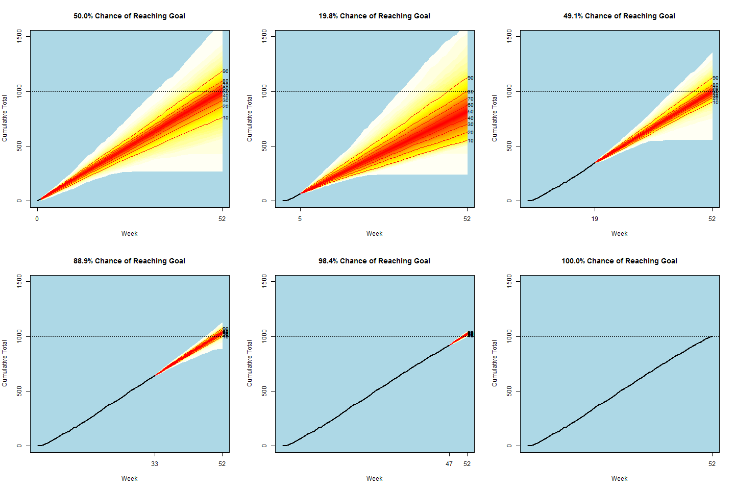
Being a data scientist, I decided to model my chance of success. The gif at the top of the page displays the simulated cumulative paths based on my final Bayesian model. The path results were updated after each passing week. I provide a description of my final model which can be found in the last section below for anyone interested. My data, code, and some output from the analysis can be found here.
What I learned from all this?
I. Hate. Running. Although I accomplished my fitness goal and ended with 1001 miles, it’s very unlikely I will run 1000 miles in a year ever again. The time commitment was a little more than I had anticipated and the repetitive exercise led to problems with my physical health. After 900 miles or so I developed a stress fracture in my right ankle which took ~6 months to heal. The lengthy recovery is likely due to the fact that I ran the last ~100 miles in pain just for the sake of accomplishing my goal. I’ll take stubbornness for the win.
What I Tried
My first idea was to try a Bayesian structural time series approach to forecasting the weekly run total, which then would be aggregated into the cumulative total. I had been reading about several R packages (bsts,CausalImpact) which had recently been released by researchers at Google. The out-of-the-box versions of these packages assumed a Gaussian model which unfortunately led to inconsistent results for my real world running data. The below figure was generated using the bsts package after 17 weeks of running. You’ll notice the rightmost image shows the possibility of a decreasing cumulative run total, which does not make sense. Hence a constraint is required.

Since the Gaussian assumption was inconsistent with the raw run data, I tried applying the same techniques under a log-normal model. This resulted in the updated figure appearing below. Now the rightmost image shows non-decreasing paths, but contains the possibility of extremely large outcomes (e.g. run totals exceeding 1500 miles). Upon inspection, large simulated paths would commonly contain weekly run totals which exceeded 100 miles; an amount known to be unrealistic for my time and physical constraints. I tried adjusting variance hyperparameters but this explosive behavior was often present.

My Final Model
Although I was not born a Bayesian, I decided on a fairly subjective parameterization which appeared to suit my needs. Here is an overview of the framework:
- The model for a weekly run total contains a mixture of two transformed beta distributions and a catastrophic failure component.
- One transformed beta distribution corresponds to a “normal week” and is scaled to be on the interval [10,50] using the formulas for mean and variance. Here I am explicitly adding the constraint which excludes the possibility that a week has a run total in excess of 50 miles.
- The second beta distribution corresponds to a “down week” and is scaled to be on [0,20]. This represents the occurrence of a poor performance week due to injury, sickness, travel, or some other reason.
- The up/down selection was governed by a binomial with conjugate beta prior. Initially I assumed approximately 8 out of 52 weeks would be down, and the posterior probability would be updated each week. I ended up having 7 down weeks in total.
- The “normal” and “down” week beta distributions were updated using exponentially weighted moving averages (EWMA) on the observed mean and prediction variance, and then solving for the appropriate beta parameters to match the transformed mean and variance. The EWMA coefficients were selected sequentially by minimizing sum of squared errors on past data.
- The catastrophic failure component reflects the chance a major event occurs which leads to early quitting (break leg, blowout knee, lose hope). I subjectively set this to have a 5% chance of happening at some point during the year.
- The final hyperparameters were set to match my initial 50/50 view of success.
Each week I updated the model parameters based on the latest data, and then would simulate 1000 run total paths. These weekly simulations were used to generate the below gif. You’ll notice I started off slowly and had to play catch-up for the first half of the year.
